Dyco est une équipe du laboratoire LIED de l université de Paris qui s intéresse à la thermodynamique hors d équilibre et à ses conséquences sur le monde qui nous entoure
Dyco est une équipe du laboratoire LIED de l université de Paris qui s intéresse à la thermodynamique hors d équilibre et à ses conséquences sur le monde qui nous entoure
This work has been developped in collaboration Maxime Massoudzadegan (massoudzadegan.maxime@gmail.com), in collaboration with Michel Piat (APC, UMR 7164) and Faouzi Boussaha (GEPI, UMR 8111)
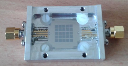
Les MKIDS sont des capteurs supraconducteurs, (Al ou Nb) dédiés à la détection de photons de basse énergie, par brisure de paires de Copper dont l’énergie de liaison est voisine de celle des photons recherchés. La mesure est basée sur le décalage fréquentiel d’un oscillateur LC dont l’inductance, appelée inductance cinétique, est fonction du gap des paires, mais aussi de la résistivité de la phase électronique dans l’état normal. Il est possible de modifier cette inductance, par un dépôt de métal (Au) sur la couche active, afin, par effet de proximité, de modifier la densité électronique localement. Des travaux sont actuellement en cours en partenariat avec les laboratoires APC (Michel Piat), et GEPI- OBSPM (Faouzi Boussaha) [1].
[1] H. Jie, M. Salatino, A. Traini, C. Chaumont, F. Boussaha, C Goupil, M. Piat, Proximity-Coupled Al/Au Bilayer Kinetic Inductance Detectors, J Low Temp Phys (2020) doi:10.1007/s10909-019-02313-4
Mesoscopic physics is a field of physics that describes systems whose dimensions range from quantum mechanics to classical mechanics. In this field, which is at the interface between quantum mechanics, electronics and thermodynamics, theories have been developed to explain the transport of charges in matter in systems with dimensions in the range of 100nm to 1000nm. In this document, we will describe the transport of loads, particularly in a system composed of a so-called normal metal and a so-called superconductive metal. Since our system consists of a superconductor, we need to expand our theoretical field to explain the superconductive part of our system with a theory known as BCS (Bardeen, Schriefer, Copper). Indeed, in a superconductor, electrons form pairs called Cooper pairs; a phenomenon explained by L. Cooper to explain the superconducting nature of matter. When the material becomes superconducting, a gap \(\Delta\) opens and it is in this gap that Cooper’s pairs live. The part of the device that will interest us is the interface between normal metal and superconducting metal. At the interface, a result of the BCS theory presents the behaviour of an incident electron at the normal-superconductor interface with a special reflection: Andreev’s reflection. Indeed, when an electron from the normal part arrives with an energy lower than the superconductor gap \(\Delta\) at the interface, it transmits a pair of Cooper in the superconductor part. De facto, by keeping the spin a hole is reflected in the normal part. This process is called Andreev’s reflection.
The objective is to determine the scaterring matrix associated with the normal-superconductor interface in order to have access to measurable and usable quantities for technologies using this type of junction such as intensity and conductance.
Attention: It is important to know that what we present in this document is valid only by considering a disruptive theory. Indeed, it has been shown, in a non-disruptive way, that if we take any state of the normal part (i. e. a vector in the Hilbertian space of the normal part) and any state of the superconducting part (i. e. a vector in the Hilbertian space of the superconducting part) and make the scalar product between them, we obtain zero. This means that the two spaces are not connected and that there is, a priori, no theoretical link between the normal and superconducting parts. This singularity is due to the fact that the phenomenon of superconductivity is due to a second-order phase transition; indeed, matter does not change state but the behaviour of electrons in superconducting matter is completely different when the material is in its normal state. It is in this context that disruptive considerations have been considered, in particular by considering a potential interface between the normal and superconducting parts to explain what we are experimentally observing in order to be able to draw results on normal-superconducting hybrid systems.
We are now going to determine the scaterring matrix of the metal-superconductor interface. To do this, we will use the Bogolyubov-Gennes matrix to arrive, after algebraic calculations on the scaterring matrix associated with the normal-superconductive interface. Bogolyubov-de Gennes equations are equations that describe the behaviour of electrons and holes in normal and superconducting metals. They are in this form:
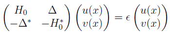
Where \(H_{0} = \frac{(\vec{p} + e\vec{A})^{2}}{2m} + V - E_{F}\) and \(\Delta = \Delta_{0} \exp{(i \phi)}\). \(H_{0}\) is the electron’s Hamiltonian containing the electrostatic potential \(V\) and the vector potential \(\vec{A}\). In addition, the energy \(\epsilon\) of the charge carriers are measured against the Fermi energy \(E_{F}\). \(\Delta\) is a running function that is zero in the normal part and is worth \(\Delta_{0}\exp{(i\phi)}\) in the superconducting part. In addition, this energy represents the matching energy of the Cooper pairs in the superconducting part. The system we are studying is composed of a normal metal and a superconducting metal as shown in the figure.
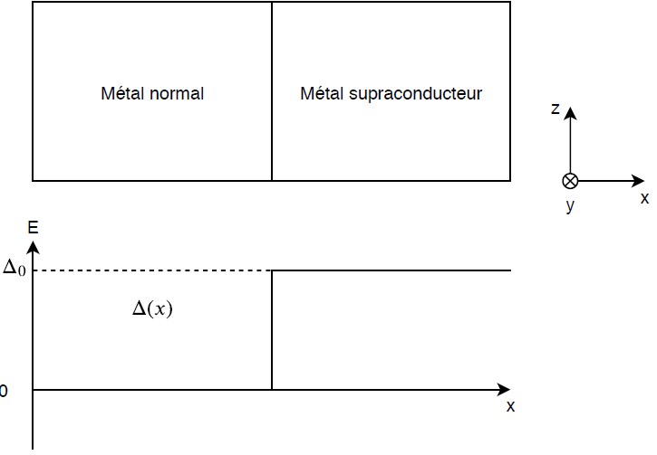 Normal metal-superconducting metal system
In the following section we will describe how the transport of charge carriers is carried out at the interface of the superconductor and the normal metal through the scaterring matrix associated with the interface.
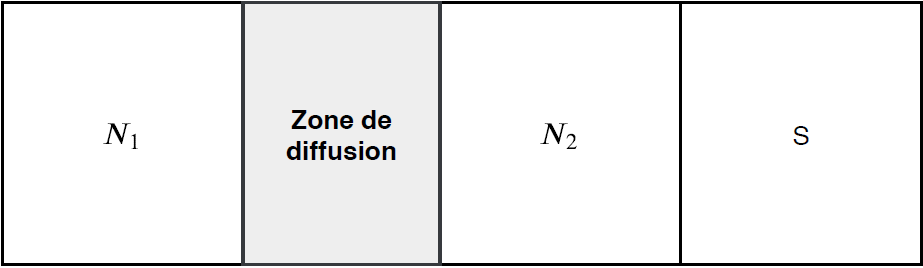
To construct the scaterring matrix, we must locate the scattering area in which we can calculate transmission, reflection and conductance coefficients. Since a scaterring matrix only makes sense in a diffusive system, the simplification we do is that we consider two parts in normal metal: a first part that is not in contact with the superconductor and a second part that is in contact with the superconductor and will therefore be affected by it. The space between the two will therefore be the diffusive zone that will be described by the scaterring matrix. We can do this simplification of two regions in the normal part, within the limit where the average free path of the charge carriers in the superconductor is large compared to the coherence length \(\xi\), which is the characteristic length of the variation in the density of the charge carriers superconductor.
In this document we consider a magnetic field \(\vec{B}\) in the direction of \(z\). You can choose a gauge for the vector potential; \(\vec{A}=\vec{0}\) in the part \(N_{2}\) and \(S\) and \(A_{x}=A_{y}=0, A_{y}=A_{1}=constant\) in the part \(N_{1}\). We also recall that \(\Delta=0\) in the normal part.
We will first calculate the wave functions of charge carriers, i. e. electrons and holes, in normal parts 1 and 2.
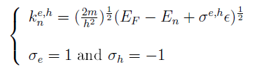
In the previous section, we have set the physical conditions in each part of the system. This part being calulatory, only the results will be given:
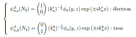
In this part we have \(\Delta=0\) and \(\vec{A}=\vec{0}\). We take the Bogolyubov-de Gennes equations and solve the differential equations to find a set of wave functions: a first part describing the electrons and another part describing the holes.
In this part we have \(\Delta=0\) and \(\vec{A}=A_{1}\vec{y}\). Similarly, we take the Bogolyubov-de Gennes equations and solve the differential equations to find another set of wave functions: a first part describing the electrons and another part describing the holes.
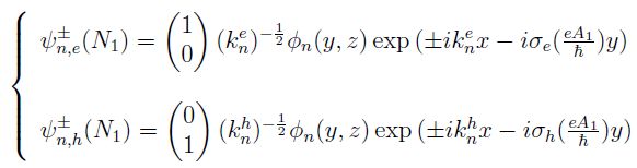
For the two regions we have:
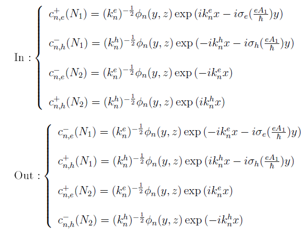
In the following section we will use the wave function coefficients we found above to form the scaterring matrix associated with the normal-superconductor interface.
First, let’s identify the coefficients of the incoming and outgoing waves:
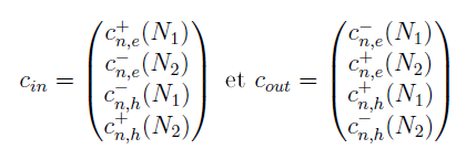
With these coefficients, we can now construct the two vectors that will be linked by the scaterring matrix:
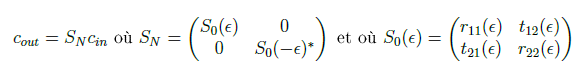
The equation of the scaterring matrix is presented as the equation \ref{eq: equation scaterring}. Note that the inverse diagonal of \(S_{N}\) is zero. This is because in the normal part, electrons and holes are not coupled.
Before continuing the development of the matrix, we must ask ourselves in what energy configuration we are in to have an Andreev reflection between the normal metal and the superconducting metal. It has been shown that Andreev’s reflection takes place when \(0<\epsilon<\Delta_{0}\).In addition, we are within the limit of \(\Delta_{0}<<E_{F}\); this approximation is called Andreev’s approximation. Under these conditions, there is no propagation mode in the superconductor. We can define a scaterring sub-matrix in the region \(N_{2}\): this scattering sub-matrix can be interpreted as the scaterring matrix of Andreev’s reflection between the region \(N_{2}\) and \(S\). This sub-matrix links the vector (\(c_{n,e}^{-}(N_{2})\),\(c_{n,h}^{+}(N_{2})\)) and the vector (\(c_{n,e}^{+}(N_{2})\),\(c_{n,h}^{-}(N_{2})\)). This was possible by linking the wave functions of the \(N_{2}\) region with the functions of the \(S\) region. The following relationships are obtained:
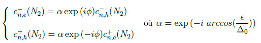
We can make two observations on these results. The first is that we can observe a phase shift of \(-arccos(\frac{\epsilon}{\Delta_{0}})\). This shift is due to the fact that the wave function of the charge carrier arriving from the region \(N_{2}\) enters the superconductor. The second observation is the positive or negative shift of \(i\phi\): indeed, we have \(i\phi\) when reflecting from a hole to an electron and \(-i\phi\) when reflecting from an electron to a hole.
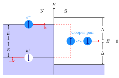
Energy diagram of an Andreev reflection
After having set up this energy environment, we can continue the development of the total scaterring matrix of our system and above all be able to make significant simplifications.
We have the following relationships:
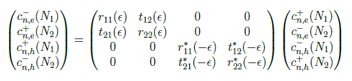
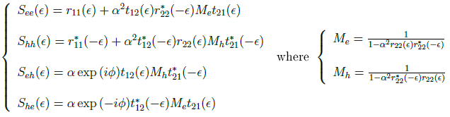
According to the equations, we can replace \(c_{n,e}^{-}(N_{2})\) and \(c_{n,h}^{+}(N_{2})\) to obtain, after some algebraic calculations, a 4x4 final scaterring matrix:

with